CBCT Basics: How to Read a Dental CBCT Scan

A CBCT scan is one volume with several ways to look at it. Most reading mistakes come from a few settings: which plane you’re on, how the window is set, how thick the slice is, and where the line you drew actually runs. The five-minute lesson walks through each of them on real scans, and every image in it is computed from the scan data.

The volume and the field of view

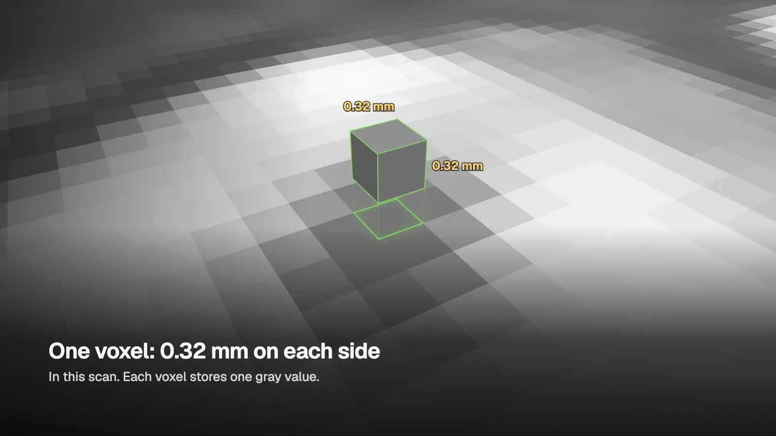
The scanner rotates around the head, captures hundreds of projections and reconstructs them into a block of voxels. Each voxel is a small cube that stores one gray value. In the head phantom used for most of the lesson, a voxel is 0.32 mm on each side, and the volume holds 471 × 471 × 441 of them, about 97.8 million voxels.

Field of view is the size of that block, written as diameter by height in millimeters (Ø × H). Choose the smallest field that answers the clinical question, which keeps the dose as low as diagnostically acceptable (ALADA). The field of view guide matches common fields to case types.

Axial, coronal and sagittal

Three planes cut the same volume. Axial is the horizontal slice, the view for bucco-lingual width and for where roots, implants and impactions sit. Coronal faces the patient and shows height and side-to-side relationships, such as ridge height under the sinus. Sagittal is the side view, front to back and top to bottom. Most viewers draw each plane as a colored reference line in the other two panes, so you can always see where a slice sits.

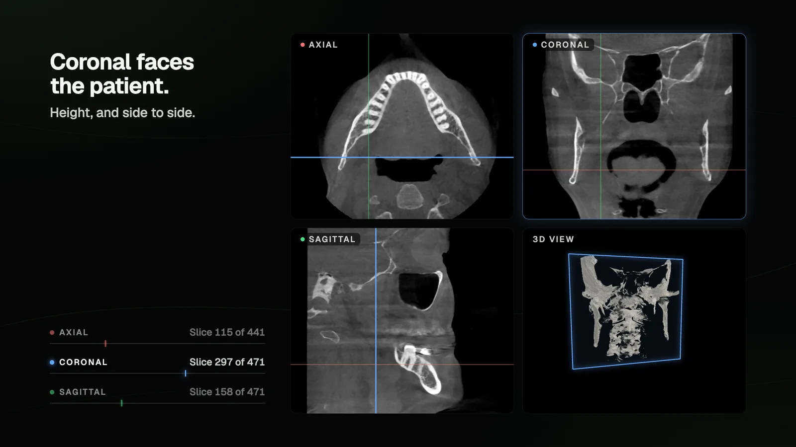
The 3D render is for orientation and for walking a patient through a case. Measure on slices. A rendered surface moves when its threshold changes, so a measurement taken on a render depends on a display setting. A periapical stays sharp but stacks every layer of anatomy into one image, where a CBCT slice shows a single layer.

Window and level

Window width sets contrast and window level sets brightness. Narrow the width and fewer gray values spread from black to white, so contrast rises. Raise the level and the image darkens, because more of the volume falls below black. A soft-tissue window and a bone window are two displays of the same scan, and the data never changes.

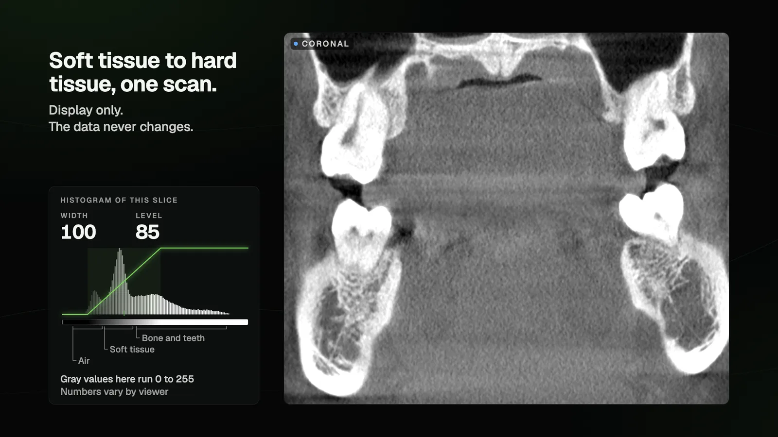
CBCT gray values aren’t calibrated Hounsfield units. In the lesson, two points in the same air space read 42 and 33 on a 0 to 255 scale. Use gray values to separate structures within a scan, and avoid reading them as bone density or comparing numbers between machines and viewers.

Slice thickness

The thinnest slice is one voxel. Thicken it and the viewer averages every slice inside the slab, so each pixel becomes the mean of its stack. Noise averages out, and anatomy from the whole slab stacks up in the image.

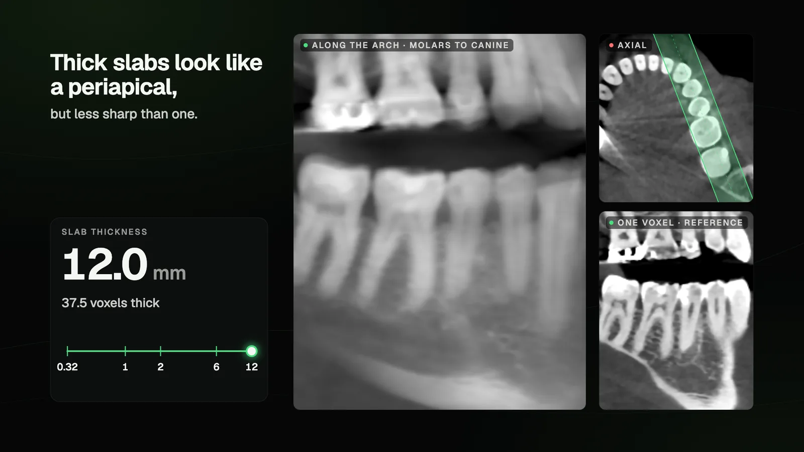
Lay a 10 to 12 mm slab along the posterior teeth and it reads much like a periapical, though without a periapical’s line-pair resolution. Go thin when the detail is small. A canal that shows on a 0.1 mm slice averages away in a 3 mm slab.

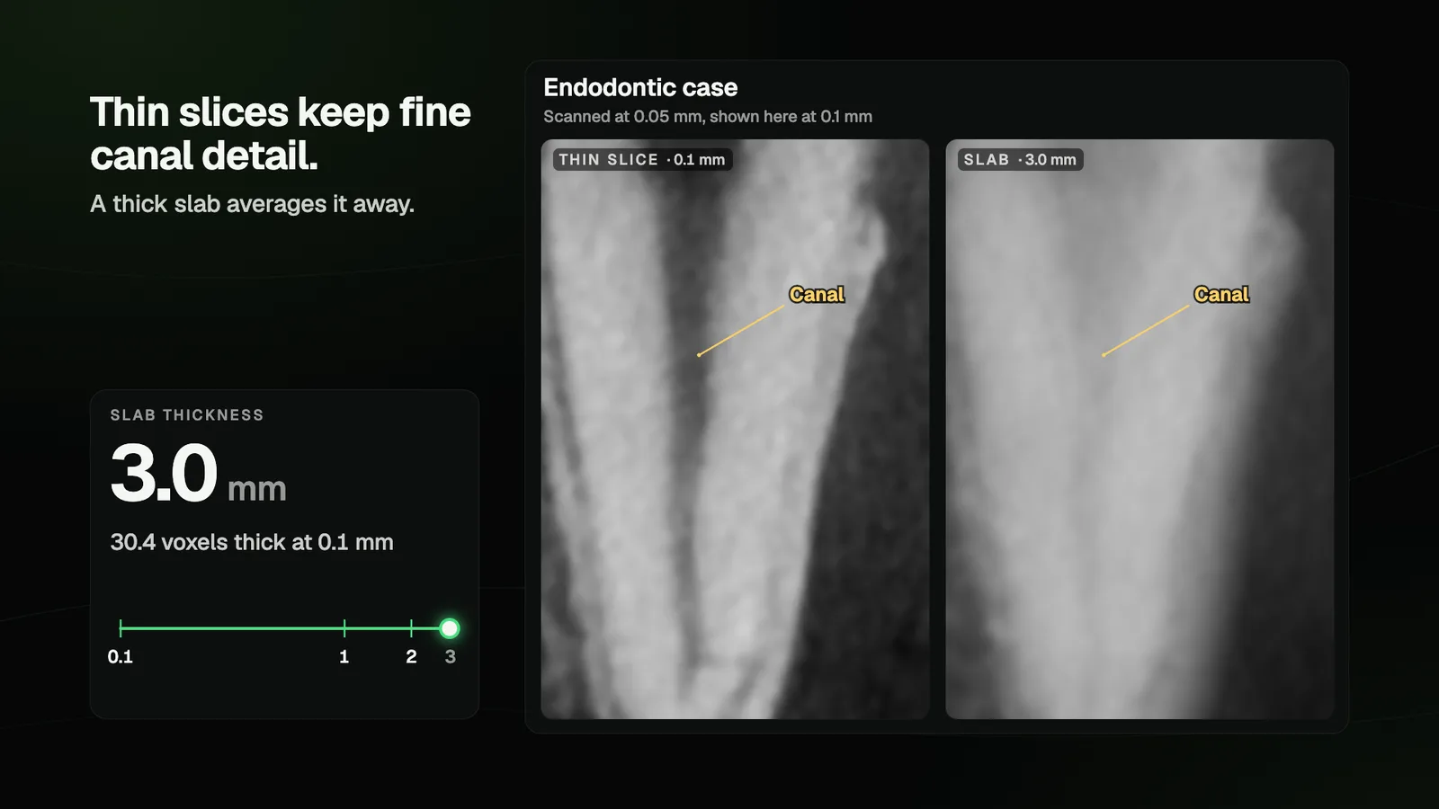
Thickness is a viewing setting. You choose it on screen after the scan, so changing it adds no dose and no scan time. Dose is set at acquisition, by the protocol and the field of view.

Curved MPR and the reconstructed panoramic

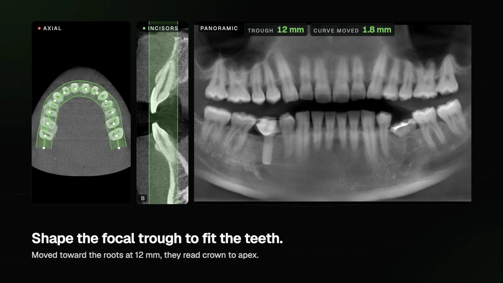
Trace a curve along the arch on an axial slice and the software builds a panoramic from the same volume. Each column of that image averages a slab across your curve, its focal trough. Proclined front teeth can lean out of a trough that stands straight up, and their roots fade. Move the front of the curve toward the roots, or stack a few more millimeters of thickness, and the anterior teeth read crown to apex.

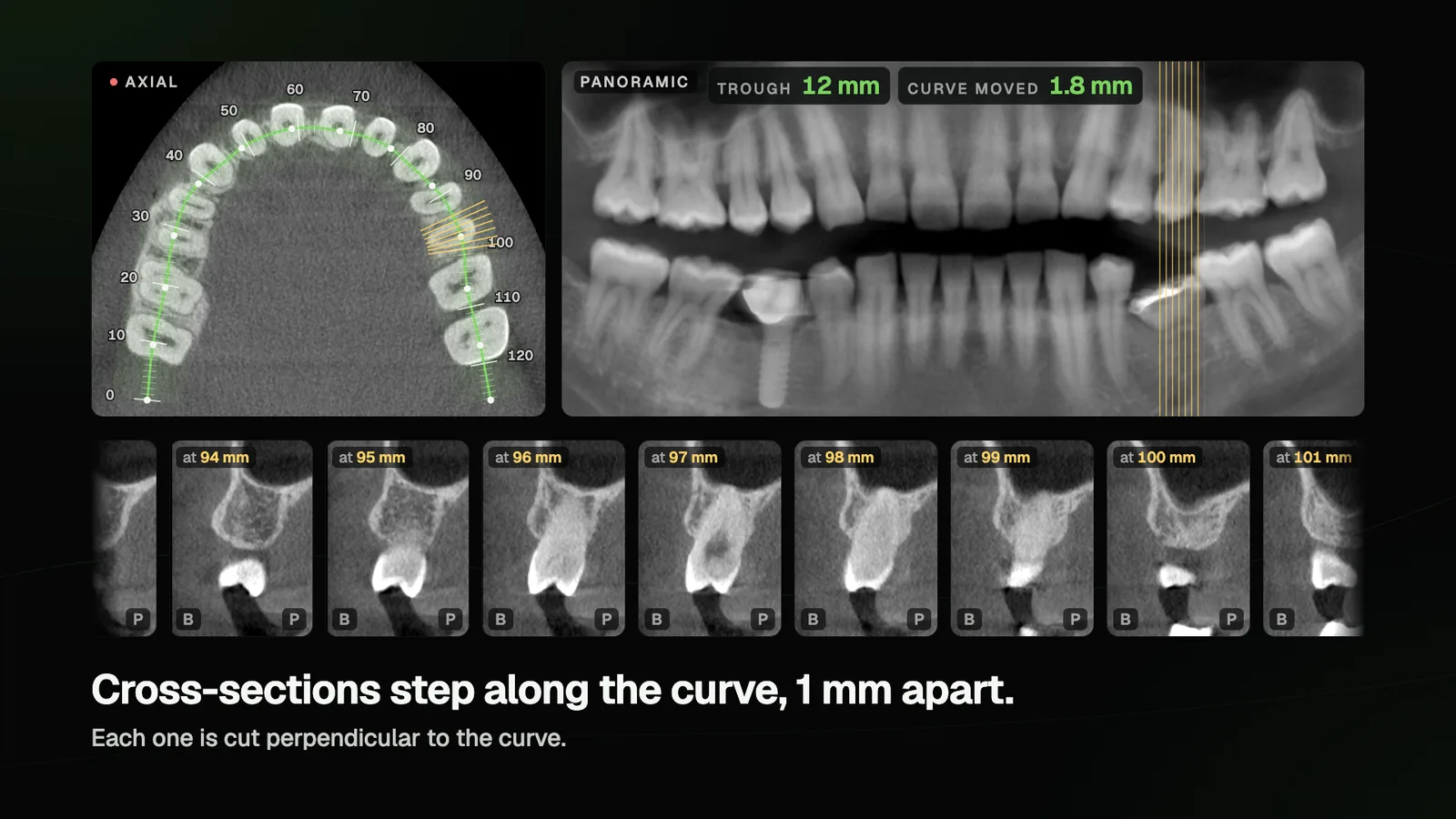
Cross-sections then step along the curve at a set spacing, 1 mm in the lesson, each one cut perpendicular to the curve. Name a series by the direction it steps. Along the arch, sections step mesial to distal and each one is bucco-lingual. Draw a line from buccal to palatal instead and they step along that line, each one mesio-distal. Radial planes turn around a tooth’s long axis to show each root, and slices across that axis climb from root to crown. Tools like these are built into i-Dixel and One Volume Viewer, and MPR curves in i-Dixel shows them on screen.

Measure on the true long axis

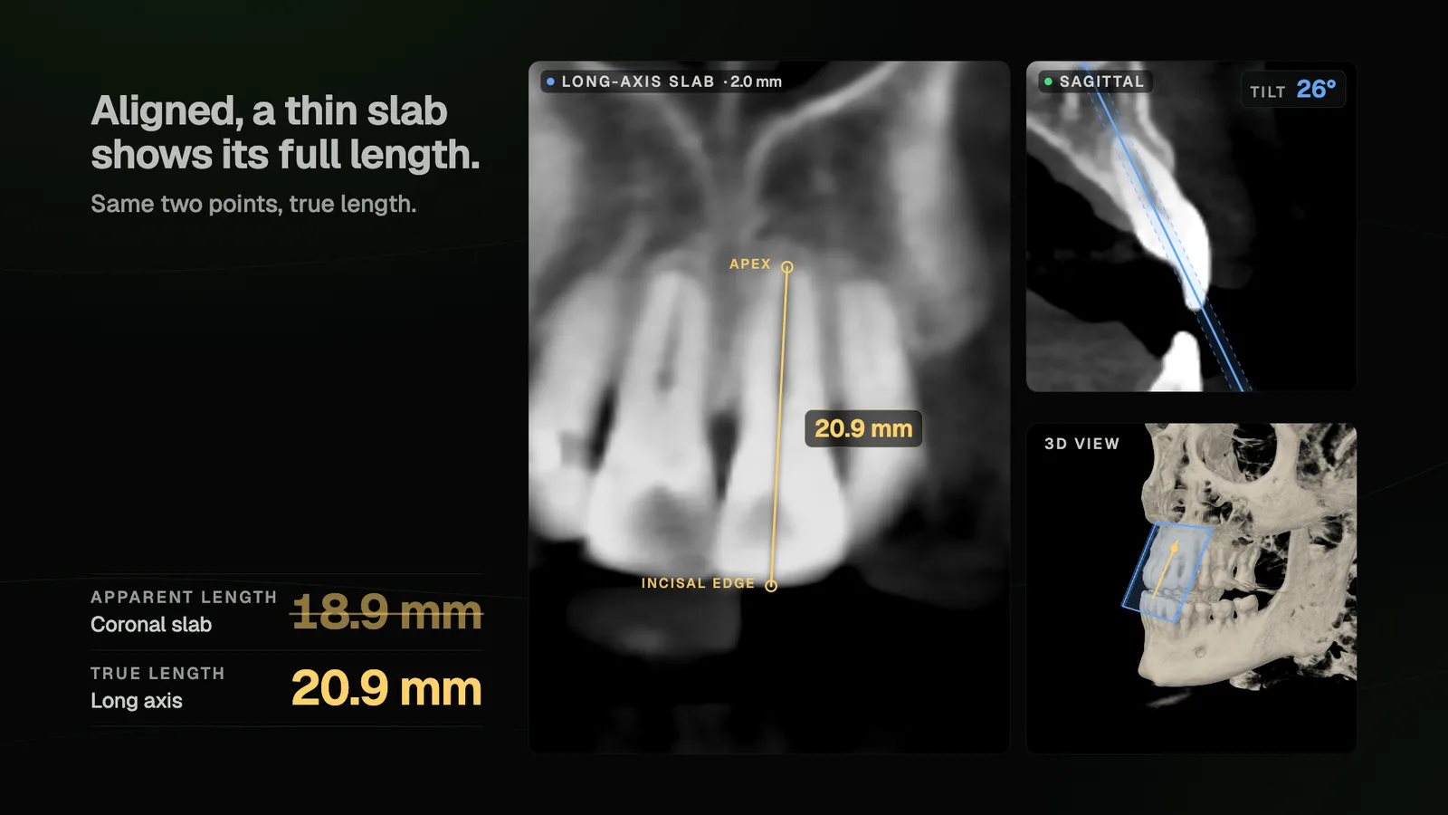
A slice that crosses a tooth at an angle foreshortens it. In the lesson, an incisor measured 18.9 mm on a coronal slab that crossed it at 26°. With the slab lined up on the tooth’s long axis, it measured 20.9 mm. Before you measure a root, a canal or an implant site, rotate the reference lines until the slice runs along the structure.

Landmarks and metal artifacts

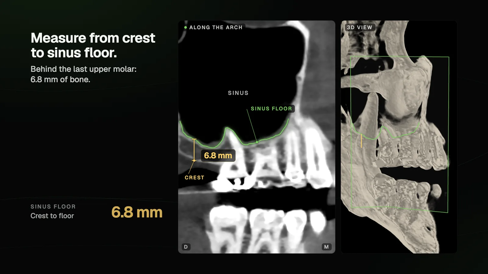
Map the landmarks before you plan: the mental foramen and the mandibular canal in the posterior mandible, the sinus floor in the posterior maxilla. Measure from the crest to the landmark on a slice that follows the tooth row.

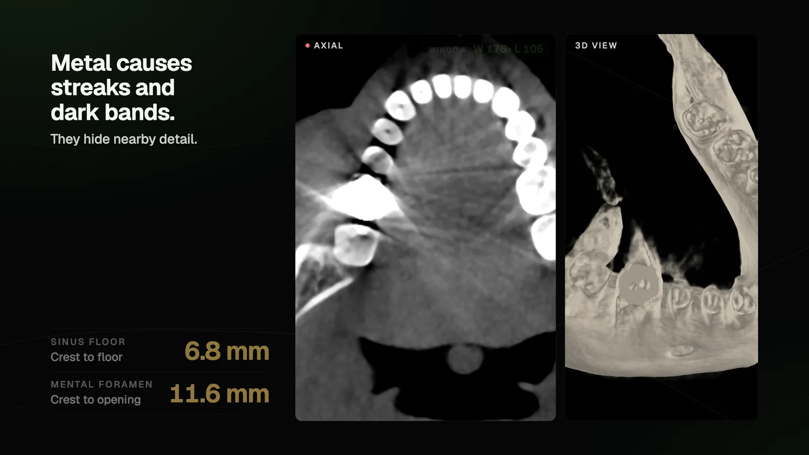
Metal throws streaks and dark bands that hide nearby detail, so read the anatomy next to crowns, posts and implants with extra care. Some systems are built to reduce it. The J. Morita X800 scans with a horizontal beam, the PreXion Excelsior line offers three-level MAR, and the HDX Will Eco-X and Dentri Max include Precision MAR. All of them are among the CBCT systems we carry.

Check an implant site in both directions

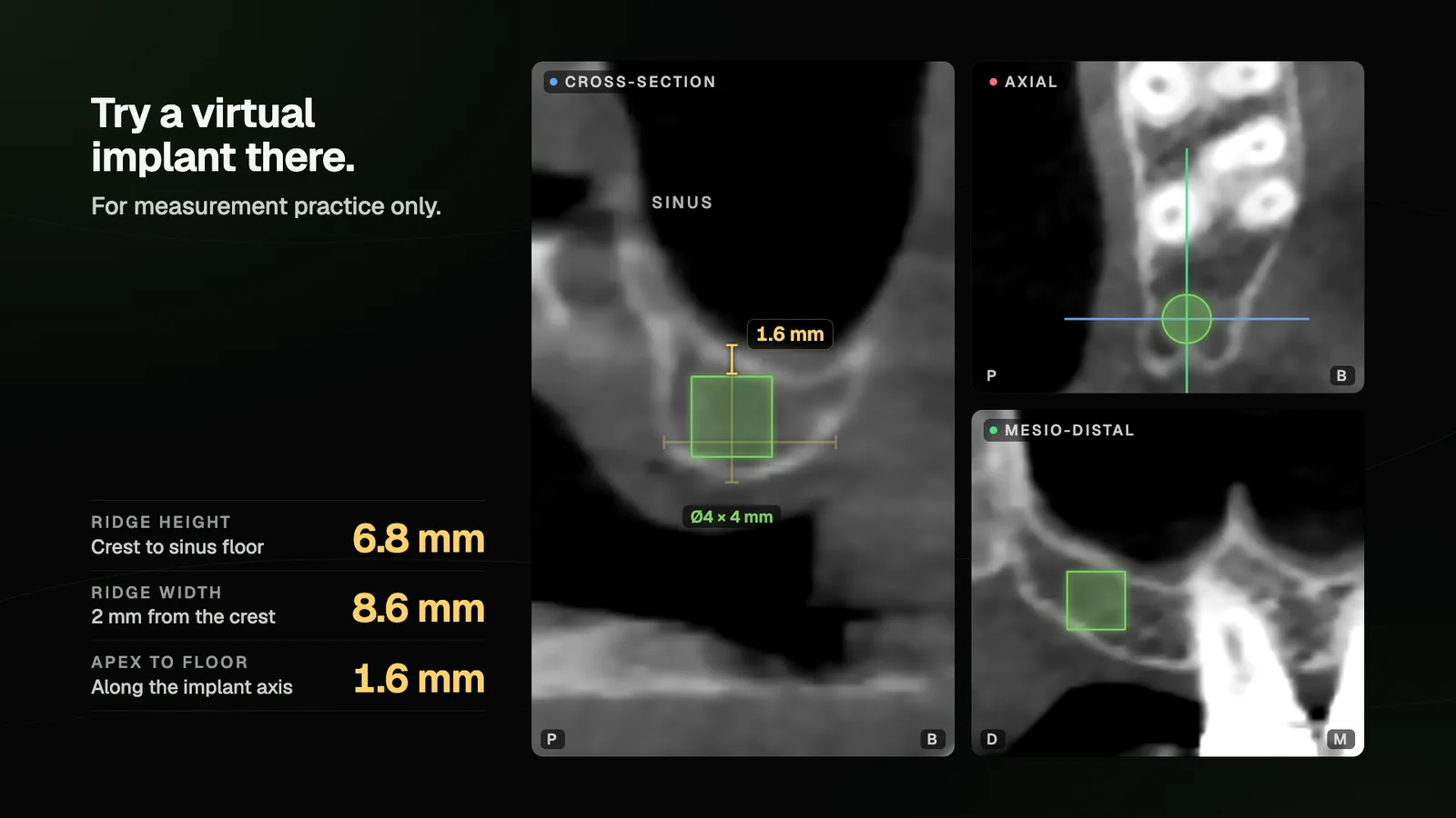
Measure ridge height and width on a cross-section first. At the lesson’s site behind the last upper molar of the head phantom, the ridge measures 6.8 mm from crest to sinus floor and 8.6 mm wide 2 mm below the crest. Then place a virtual implant and step through it slice by slice in both stacks. A 4 × 4 mm test cylinder there clears the sinus floor by 1.6 mm along its axis, yet the mesio-distal stack shows its apex meeting the floor mesially, which the bucco-palatal stack alone would miss. The cylinder is a measuring exercise on a phantom.

Export and share

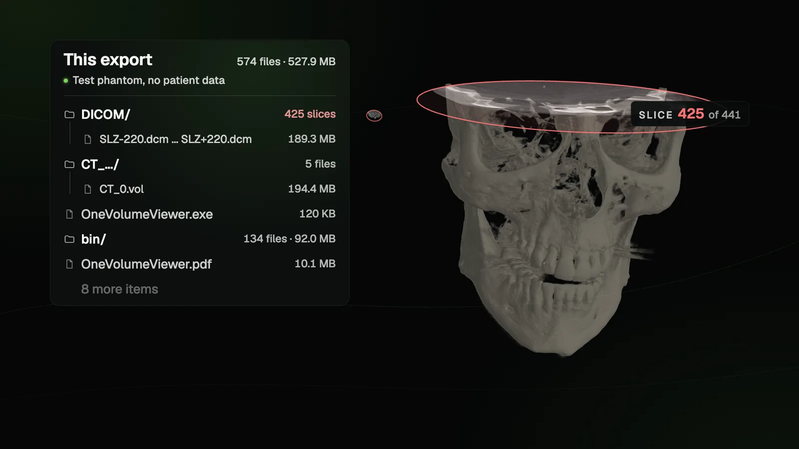
Labs and planning software need DICOM. A patient needs the volume with a viewer they can open, so learn both export paths in your software. The phantom export in the lesson holds a DICOM folder with one file per axial slice, the volume file and One Volume Viewer. Send any scan through a HIPAA-compliant service that signs a business associate agreement (BAA).

Reading CBCT gets faster with practice on your own scans, and expert support is a phone call away when one raises a question.